Bertaina and Giorgini, Phys. Rev. Lett. 106, 110403 (2011)
Ref. [20] uses fixed-node diffusion Monte Carlo.
Table I provides energies with uncertainties.
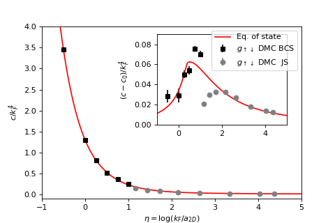
Figure 4 shows the contact density \(c/k_F^4\). The data were provided by Gianluca Bertaina.
- tdg.references.PRL106110403.table_I()[source]
Note that Fig. 2 shows 18 points but Table I gives only 16 rows.
- Returns
torch.tensor
- Return type
The rows are \(\ln(k_F a_{2D})\), \(E/E_{FG}\), the uncertainty on \(E/E_{FG}\), and half the binding energy \(\mathcal{E}_B\).
- tdg.references.PRL106110403.conventional_table_I()[source]
The same as
table_I()but converted from the geometric convention.
- tdg.references.PRL106110403.figure_4()[source]
Figure 4 of Ref. [20] provides measurements of
contact_by_kF4()as a function of \(\log k_F a_{2D}\).Returns the data from Figure 4, in TWO tensors, the first with BCS data and the other with JS data. Each tensor has \(\log k_F a_{2D}\) in the first row, \(c/k_F^4\) in the second, and the uncertainty on \(c/k_F^4\) in the third.
The data were provided by Gianluca Bertaina.
- tdg.references.PRL106110403.c0_by_kF4(eta)[source]
Explained just above Figure 3, \(c_0\) is ‘the contribution to the contact from the molecular state’.
- Parameters
eta (torch.tensor) – \(\eta = \log k_F a_{2D}\)
- Returns
The two-body contribution to the contact at \(\eta\).
- Return type
torch.tensor
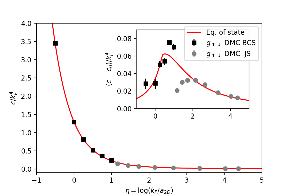
- tdg.references.PRL106110403.figure_4_fit(eta)[source]
Figure 4 of Ref. [20] shows a fit of
contact_by_kF4()as a function of \(\log k_F a_{2D}\).The fit parameters were provided by Gianluca Bertaina.
- Parameters
eta (torch.tensor) – \(\eta = \log k_F a_{2D}\)
- Returns
\(c/kF^4\) at \(\eta\).
- Return type
torch.tensor
- tdg.references.PRL106110403.figure_4_reproduction(ax)[source]
Reproduce Figure 4 of Ref. [20] relying on data in
figure_4()and thefigure_4_fit().import matplotlib.pyplot as plt fig, ax = plt.subplots(1,1, figsize=(6,4)) from tdg.references import PRL106110403 ax, inset = PRL106110403.figure_4_reproduction(ax)
(
Source code,png,hires.png,pdf)
- Parameters
ax (matplotlib.Axes) – Where to draw the figure.
- Returns
ax (matplotlib.Axes) – The same handle given, but with art.
inset – A handle for the inset.
- tdg.references.PRL106110403.conventional_figure_4()[source]
The same data as
figure_4()but with \(\log k_F a\) rather than \(\log k_F a_{2D}\).