Hybrid Monte Carlo

Hybrid Monte Carlo [10], HMC, or Hamiltonian Monte Carlo, is an importance-sampling algorithm with origins in lattice field theory. Given a real

tdg.HMC.Hamiltonian

class tdg.HMC.Hamiltonian(S)[source]

Bases: H5able

The HMC Hamiltonian for a given action \(S\) is

\[\mathcal{H} = \frac{1}{2} p M^{-1} p + S(x)\]

which has the standard non-relativistic kinetic energy and a potential energy given by the action.

An HMC Hamiltonian serves two purposes:

The first is to draw momenta and evaluate the starting energy, and to do accept/reject according to the final energy. For this purpose Hamiltonians are callable.
The second is to help make a proposal to consider in the first place. To do this we start with a position and momentum pair and integrate Hamilton’s equations of motion,

\[\begin{aligned} \frac{dx}{d\tau} &= + \frac{\partial \mathcal{H}}{\partial p} & \frac{dp}{d\tau} &= - \frac{\partial \mathcal{H}}{\partial x} \end{aligned}\]

Of course, these two applications are closely related, and in ‘normal’ circumstances we use the same Hamiltonian for both purposes.

__call__(x, p)[source]

Parameters

x (torch.tensor) – a configuration compatible with the Hamiltonian
p (torch.tensor) – a momentum of the same shape

Returns

\(\mathcal{H}\) for the given x and p.

Return type

torch.tensor

T(p)[source]

velocity(p)[source]: The velocity is needed to update the positions in Hamilton’s equations of motions.

\[\texttt{velocity(p)} = \left.\frac{\partial \mathcal{H}}{\partial p}\right|_p\]

force(x)[source]: The force is needed to update the momenta in Hamilton’s equations of motions.

\[\texttt{force(x)} = \left.-\frac{\partial \mathcal{H}}{\partial x}\right|_x\]

tdg.HMC Integrators

Practically, integrating Hamilton’s equations of motions for a finite amount of molecular dynamics time md_time requires discretizing the fictitious time into an integer number of md_steps and choosing a numerical method. Integrators trace trajectories through the phase space of the auxiliary fields and associated momenta.

To maintain good Markov Chain properties the integrator should be reversible; if we do not incorporate any integration Jacobian into the accept/reject step [11], we need a symplectic integrator. Two classics are the LeapFrog and Omelyan integrators.

Specifying the integrator’s discretization can be done manually. Too fine a discretization and you waste time; too coarse and the HMC energy conservation is violated too dramatically, leading to a poor acceptance rate. One can also use an Autotuner to target a particular acceptance rate.

class tdg.HMC.LeapFrog(H, md_steps, md_time=1)[source]

Bases: H5able

The LeapFrog integrator integrates Hamilton’s equations of motion for a total of \(\tau\) molecular dynamics time md_time in a reversible, symplectic way.

It discretizes \(\tau\) into md_steps steps of \(d\tau\) and then uses simple finite-differencing.

One step of \(d\tau\) integration is accomplished by

updating the coordinates by \(d\tau/2\)
updating the momenta by \(d\tau\)
updating the coordinates by \(d\tau/2\).

However, if the number of steps is more than 1 the trailing half-step coordinate update from one step is combined with the leading half-step coordinate update from the next.

integrate(x_i, p_i)[source]

Integrate an initial position and momentum.

Parameters

x_i (torch.tensor) – a tensor of positions
p_i (torch.tensor) – a tensor of momenta

Returns

x_f (torch.tensor) – a tensor of positions,
p_f (torch.tensor) – a tensor of momenta
log_det_J (torch.tensor) – the phase-space Jacobian = 1 since the LeapFrog integrator is symplectic; its determinant is also 1, so its log is 0.

__call__(x_i, p_i)[source]: Forwards to integrate.

class tdg.HMC.Omelyan(H, md_steps, md_time=1, zeta=0.193)[source]

Bases: H5able

The Omelyan integrator is a second-order integrator which integrates Hamilton’s equations of motion for a total of \(\tau\) molecular dynamics time md_time in a reversible, symplectic way.

It discretizes \(\tau\) into md_steps steps of \(d\tau\) and given \(0\leq\zeta\leq 0.5\) applies the following integration scheme:

Update the coordinates by \(\zeta\;d\tau\),
update the momenta by \(\frac{1}{2}\; d\tau\),
update the coordinates by \((1-2\zeta)\;d\tau\),
update the momenta by \(\frac{1}{2}\; d\tau\),
update the coordinates by \(\zeta\;d\tau\).

However, if the number of steps is more than 1 the trailing coordinate update from one step is combined with the leading coordinate update from the next.

If nothing is known about the structure of the potential, the \(h^3\) errors are minimized when \(\zeta \approx 0.193\) [12].

When \(\zeta=0\) this reproduces the momentum-first leapfrog; when \(\zeta=0.5\) it reproduces the position-first LeapFrog.

integrate(x_i, p_i)[source]

Integrate an initial position and momentum.

Parameters

x_i (torch.tensor) – a tensor of positions
p_i (torch.tensor) – a tensor of momenta

Returns

x_f (torch.tensor) – a tensor of positions,
p_f (torch.tensor) – a tensor of momenta
log_det_J (torch.tensor) – the phase-space Jacobian = 1 since the Omelyan integrator is symplectic; its determinant is also 1, so its log is 0.

__call__(x_i, p_i)[source]: Forwards to integrate.

It can be painfully time consuming to pick a good md_steps. One can try to automatically find a good molecular dynamics discretization instead.

class tdg.HMC.Autotuner(HMC_Hamiltonian, integrator, *, cfgs_per_estimate=5, _bootstrap_resamples=100)[source]

Bases: H5able

An Autotuner seeks for a molecular dynamics discretization, targeting a given acceptance rate. Based on the simple ideas explained in Reference [13].

Parameters

HMC_Hamiltonian (tdg.HMC.Hamiltonian) – The HMC_Hamiltonian is used for molecular dynamics integration and accept/reject. In principle these can be different, but that is not implemented here.
integrator (a molecular dynamics integrator) – Could be tdg.HMC.LeapFrog, tdg.HMC.Omelyan, or another integrator which just has one molecular dynamics discretization scale and is constructed via integrator(HMC_Hamiltonian, md_steps, md_time) where a good value for md_steps is what we seek.
cfgs_per_estimate (int) – How many trajectories are needed get a good estimate of the acceptance rate? Reference [13] found that (for the Hubbard model on the honeycomb lattice, but for very large lattices near the continuum limit) as few as 5 could produce a good estimate, while they never needed more than about 30.

target(target_acceptance=0.75, start='hot', md_time=1.0, starting_md_steps=20, min_md_steps=1, progress=<function _no_op>)[source]

Runs the autotuning process to achieve a target acceptance rate.

The autotuning process seeks to adjust the number of molecular dynamics steps per trajectory to achieve a specific acceptance rate (target_acceptance). It iteratively computes trajectories with different discretizations until the acceptance rate meets the target. The autotuning stops when either the target acceptance rate is achieved with some confidence or the discretization cannot be shrunk further without falling below the target.

Parameters

target_acceptance (float) – The desired acceptance rate to achieve. If the acceptance rate depends very sharply on the number of molecular dynamics steps, there may be no choice which achieves the target. In that case a finer molecular dynamics integration will be picked.
start (str, optional) – The starting condition for the autotuning process. Must be understood by generate().
md_time (float) – The time duration for each molecular dynamics trajectory.
starting_md_steps (int) – The initial number of molecular dynamics steps per trajectory.
min_md_steps (int) – The minimum number of molecular dynamics steps allowed. Default is 1.
progress (callable) – A callback function like tqdm that can be used to track HMC evolution.

Returns

integrator (molecular dynamics integrator) – An integrator object constructed with the molecular dynamics discretization tuned to the target acceptance.
configuration (torch.tensor) – The final configuration resulting from all the trajectories accepted during the tuning process, which can be used in subsequent HMC.

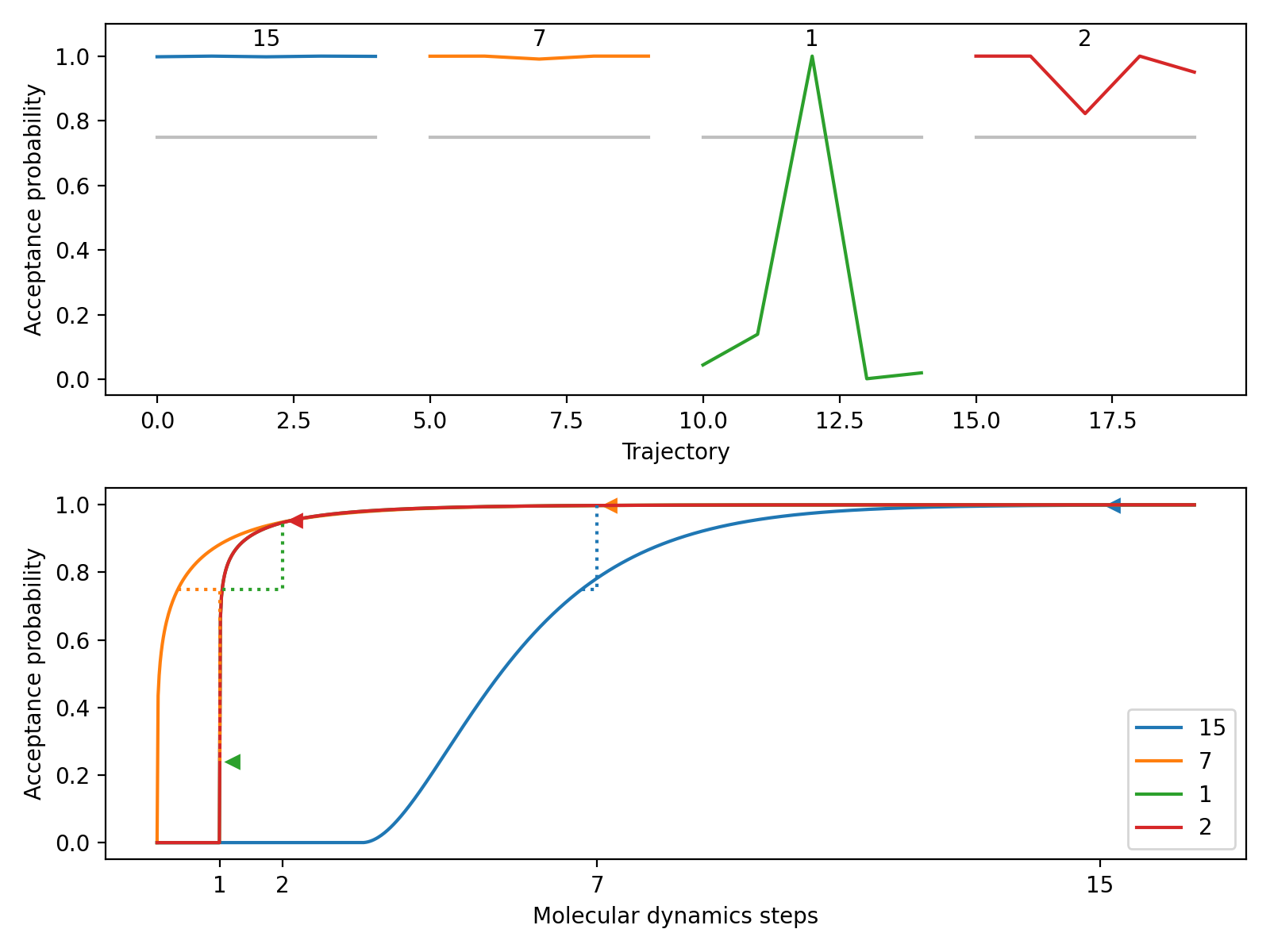
plot_history(ax, **kwargs)[source]

This method plots the acceptance probabilities over the course of the autotuning process. The acceptance probabilities are shown for each trajectory, with the x-axis representing the trajectory index and the y-axis representing the acceptance probability. The plot allows visualizing the change in acceptance probabilities over molecular dynamics time.

Parameters

ax (matplotlib.axes.Axes) – The axes on which to plot the history.
**kwargs – Additional keyword arguments to customize the plot appearance. Applied to the trace for every tuning step.

plot_models(ax)[source]

Plots the evolution of acceptance probability models with autotuning. Also shows, as points with error bars, the final estimated acceptance rates.

Parameters: ax (matplotlib.axes.Axes) – The axes on which to plot the acceptance probability models.

Here is a small and easy example which tunes relatively quickly. We start at a fine molecular dynamics discretization of 15 steps. The model then predicts 9 steps, which is found to still be fine. It jumps down to 1 step, which has poor acceptance but updates the model’s prediction to 2 steps. Testing 2 steps shows it has an acceptance rate that satisfies the autotuner.

#!/usr/bin/env python

import torch
torch.set_default_tensor_type(torch.DoubleTensor)
torch.manual_seed(9999) # for reproducibility

import matplotlib.pyplot as plt
import tdg
import tdg.HMC as HMC

S = tdg.action._demo(
        nx=9, nt=16,
        beta=0.061224489795918366, mu=torch.tensor(0.), h=torch.tensor([0., 0., 0.]),
        C0=-1.2388577106478569)
H = HMC.Hamiltonian(S)

A = HMC.Autotuner(H, HMC.Omelyan)
integrator, start = A.target(0.75, start='hot', starting_md_steps=15)

fig, ax = plt.subplots(2,1, figsize=(8,6))
A.plot_history(ax[0])
A.plot_models(ax[1])
ax[1].legend()
fig.tight_layout()
plt.show()

(Source code, png, hires.png, pdf)

# Then use the integrator and start to begin HMC...

tdg.HMC.MarkovChain

HMC is essentially a variant of the Metropolis-Hastings algorithm [14, 15]. The refreshing of the momentum and subsequent integration form a proposal machine for an accept/reject step given by the Boltzmann factor determined by the Hamiltonian \(\mathcal{H}\).

class tdg.HMC.MarkovChain(H, integrator, retry_on_nan=False)[source]

Bases: H5able

The HMC algorithm for updating an initial configuration \(x_i\) goes as follows:

Draw a sample momentum \(p_i\) from the gaussian distribution given by the kinetic piece of the Hamiltonian.
Calculate \(\mathcal{H}\) for the given \(x_i\) and drawn \(p_i\).
Integrate Hamilton’s equations of motion to generate a proposal for a new \(x_f\) and \(p_f\).
Accept the proposal according to \(\exp[-(\Delta\mathcal{H} = \mathcal{H}_f - \mathcal{H}_i - \log\det J)]\) where \(J\) is the phase-space Jacobian of the integrator.

Parameters

H (HMC.Hamiltonian) – The Hamiltonian needed in the Metropolis-Hastings accept/reject step.
integrator (a molecular dynamics integrator) – Integrates molecular dynamics trajectories to give a proposal.
retry_on_nan (boole) – Sometimes if the action is too coarse we can encounter numerical under/overflow yielding NaNs; obvious nonsense. At that point the formally correct thing to do is to terminate the Markov Chain and throw it away. But… sometimes you want to press on anyway. If True and NaN is detected in either the proposed configuration or in the change in HMC energy, just take a fresh step with a different momentum, rather than raising a ValueError. The default, in contrast, is to raise a ValueError.

step(x)[source]

Parameters

x (torch.tensor) – a configuration compatible with the Hamiltonian and integrator.

Returns

x (torch.tensor) – a similar configuration; a new configuration if the proposal was accepted, or the original if the proposal is rejected.
weight (torch.tensor) – Weight not incorporated into the accept/reject. Currently hard-coded to 1.