Background

Ultracold atomic experiments can squeeze nonrelativistic fermionic atoms in one dimension, constructing a two-dimensional Fermi gas. The leading-order effective field theory [1]

\[\begin{align} \mathcal{L} = \psi^\dagger\left(i\partial_0 + \frac{\nabla^2}{2M}\right)\psi - \frac{C_0}{2} (\psi^\dagger \psi)^2 \end{align}\]

yields a Hamiltonian

\[\begin{align} H = - \psi^\dagger \frac{\nabla^2}{2M} \psi + \frac{C_0}{2} (\psi^\dagger \psi)^2 \end{align}\]

invariant under scale and nonrelativistic-conformal transformations [2]. We can rescale our Hamiltonian by \(ML^2\), which removes the dimensions. With a lattice regulation, the result is

\[\begin{align} \tilde{H} = HML^2 = \sum_{ab} \tilde{\psi}^\dagger_a\left(\kappa_{ab} - \mathcal{V} \frac{\tilde{C}_0}{2} \delta_{ab} \right) \tilde{\psi}_b + \frac{1}{2} \sum_{ab} \tilde{n} \tilde{V}_{ab} \tilde{n}_b \end{align}\]

where \(\tilde{\psi} = \psi/\Delta x\) so that \(\{\tilde{\psi}_{a\sigma}, \tilde{\psi}^\dagger_{b\tau}\} = \delta_{ab}\delta_{\sigma\tau}\), \(\kappa\) is a lattice dispersion relation we are free to pick so long as it goes to the correct continuum limit, and \(\tilde{V}\) is a lattice-regularized interaction written as sums of terms, each a LegoSphere interaction.

The purpose of the tdg library is to compute observables of many-body systems in thermodynamic equilibrium governed by this Hamiltonian. We pursue a lattice field theory-like approach, discretizing the two-dimensional space via a regular square lattice with periodic boundary conditions.

tdg.Lattice

A lattice is a two-dimensional square grid of points, a discretization of space. For simplicity we restrict our attention to an isotropic lattice with the same number of points in each rectilinear direction; a list of coordinates() is provided. We use periodic boundary conditions, and therefore can validly mod() points into the coordinates() of the lattice. The periodic boundary conditions also inform the computation of distance_squared(), because the distance might be shorter than the naive route might suggest. A lattice knows how big a spatial vector() is and knows how to Fourier transform them via fft() and ifft().

We will use the perfect nonrelativistic dispersion relation, and therefore can use the adjacency_matrix() to construct the kinetic matrix kappa().

The lattice has translational invariance and a \(D_4\) point group.

class tdg.lattice.Lattice(nx, ny=None)[source]

Bases: H5able

dims

The dimension sizes in order.

>>> lattice = Lattice(5)
>>> lattice.dims
tensor([5, 5])

sites

The total number of sites.

>>> lattice = Lattice(5)
>>> lattice.sites
25

x

The coordinates in the x direction.

>>> lattice = Lattice(5)
>>> lattice.x
tensor([ 0,  1,  2, -2, -1])

y

The coordinates in the y direction.

>>> lattice = Lattice(5)
>>> lattice.y
tensor([ 0,  1,  2, -2, -1])

X

A tensor of size dims with the x coordinate as a value.

>>> lattice = Lattice(5)
>>> lattice.X
tensor([[ 0,  0,  0,  0,  0],
        [ 1,  1,  1,  1,  1],
        [ 2,  2,  2,  2,  2],
        [-2, -2, -2, -2, -2],
        [-1, -1, -1, -1, -1]])

Y

A tensor of size dims with the y coordinate as a value.

>>> lattice = Lattice(5)
>>> lattice.Y
tensor([[ 0,  1,  2, -2, -1],
        [ 0,  1,  2, -2, -1],
        [ 0,  1,  2, -2, -1],
        [ 0,  1,  2, -2, -1],
        [ 0,  1,  2, -2, -1]])

coordinates

A tensor of size [sites, len(dims)]. Each row contains a pair of coordinates. The order matches {X,Y}.flatten().

>>> lattice = Lattice(5)
>>> lattice.coordinates
>>> lattice.coordinates
tensor([[ 0,  0],
        [ 0,  1],
        [ 0,  2],
        [ 0, -2],
        [ 0, -1],
        [ 1,  0],
        [ 1,  1],
        [ 1,  2],
        [ 1, -2],
        [ 1, -1],
        [ 2,  0],
        [ 2,  1],
        [ 2,  2],
        [ 2, -2],
        [ 2, -1],
        [-2,  0],
        [-2,  1],
        [-2,  2],
        [-2, -2],
        [-2, -1],
        [-1,  0],
        [-1,  1],
        [-1,  2],
        [-1, -2],
        [-1, -1]])

mod(x)[source]

Mod integer coordinates x into values on the lattice.

Parameters: x (torch.tensor) – Either one coordinate pair of .shape==torch.Size([2]) or a set of pairs .shape==torch.Size([*,2]) The last dimension should be of size 2.
Returns: Each x is identified with an entry of coordinates by periodic boundary conditions. The output is the same shape as the input.
Return type: torch.tensor

distance_squared(a, b)[source]

\[\texttt{distance_squared}(a,b) = \left| \texttt{mod}(a - b)\right|^2\]

Parameters

a (torch.tensor) – coordinates that need not be on the lattice
b (torch.tensor) – coordinates that need not be on the lattice

Returns

The distance between a and b on the lattice accounting for the fact that, because of periodic boundary conditions, the distance may shorter than naively expected. Either a and b are the same shape (a single or 1D-tensor of coordinate pairs) or one is a singlet and one is a tensor.

Return type

torch.tensor

cross(a, b)[source]

The cross product of two vectors \(a \times b\). In two dimensions this is a scalar value. However, for compatibility with three dimensions we add an extra index.

Parameters

a (torch.tensor:) – first vector
b (torch.tensor:) – second vector

Return type

torch.tensor

If a and b are single vectors, returns a single value in a one-dimensional torch.tensor.

>>> lattice = Lattice(5)
>>> x = lattice.coordinates
>>> lattice.cross(x[1], x[5])
tensor([-1])

If a is a single vector and b is two-dimensional (vector index last), returns a tensor of shape [b.shape[0], 1],

>>> lattice.cross(x[1], x[1:-1:5])
tensor([[ 0],
        [-1],
        [-2],
        [ 2],
        [ 1]])

Similarly, if a is two-dimensional (vector index last), returns a tensor of shape [a.shape[0], 1],

>>> lattice.cross(x[1:-1:5], x[2])
tensor([[ 0],
        [ 2],
        [ 4],
        [-4],
        [-2]])

Finally, if both a and b are two-dimensional (vector index last), returns a tensor of shape [a.shape[0], b.shape[0], 1],

>>> lattice.cross(x[:5], x[:7]).shape
torch.Size([5, 7, 1])

coordinatize(v, dims=(-1,), center_origin=False)[source]

Unflattens all the dims from a linear superindex to one index for each dimension in .dims.

Parameters

v (torch.tensor) – A tensor with at least one dimension linearized in space.
dims (tuple of integers) – The directions you wish to unflatten into a meaningful shape that matches the lattice.
center_origin (boolean) – If true, each coordinatized dimension is rolled so that the origin is in the center of the two slices. This is primarily good for making pictures. linearize() does not provide an inverse of this, because you really should not do it in the middle of a calculation!

Returns

v but tensor more, shorter dimensions. Dimensions specified by dims are unflattened.

Return type

torch.tensor

linearize(v, dims=(-1,))[source]

Flattens adjacent dimensions of v with shape .dims into a dimension of size .sites.

Parameters

v (torch.tensor) –
dims (tuples of integers that specify that dimensions in the result that come from flattening.) – Modded by the dimension of the resulting tensor so that any dimension is legal. However, one should take care to ensure that no two are the SAME index of the result; this causes a RuntimeError.

Returns

v but with fewer, larger dimensions

Return type

torch.tensor

Note

The dims parameter may be a bit confusing. This perhaps-peculiar convention is to make it easier to combine with coordinatize. linearize and coordinatize are inverses when they get the same dims arguments.

>>> import torch
>>> import tdg
>>> nx = 5
>>> dims = (0, -1)
>>> lattice = tdg.Lattice(5)
>>> v = torch.arange(nx**(2*3)).reshape(nx**2, nx**2, nx**2)
>>> u = lattice.coordinatize(v, dims)
>>> u.shape
torch.Size([5, 5, 25, 5, 5])
>>> w = lattice.linearize(u, dims) # dims indexes into the dimensions of w, not u!
>>> w.shape
torch.Size([25, 25, 25])
>>> (v == w).all()
tensor(True)

vector(*dims)[source]

Parameters: dims (tuple) – Specifies how how many vectors to produce.
Returns: A dims-dimensional stack of linearized zero vectors.
Return type: torch.tensor

fft(vector, axis=-1, norm='backward')[source]

The Fourier transform on a linearized axis.

Parameters

vector (torch.tensor) – A vector of data.
axis – The axis along which to perform a 2D Fourier transform on the vector.
norm – A convention for the Fourier transform, one of "forward", "backward", or "ortho". The default is “backward”, to match our notes.

Returns

F(vector) with the same shape as the input vector, transformed along the axis.

Return type

torch.tensor

ifft(vector, axis=-1, norm='backward')[source]

The Fourier inverse transform on a linearized axis.

Parameters

vector (torch.tensor) – A vector of data.
axis – The axis along which to perform a 2D inverse Fourier transform on the vector.
norm – A convention for the inverse Fourier transform, one of "forward", "backward", or "ortho". The default is “backward”, to match our notes.

Returns

Inverse[F](vector) with the same shape as the input vector, transformed along the axis.

Return type

torch.tensor

inversion(vector, dims=(-1,))[source]

Reflect data across the origin for each dimension.

Parameters

vector (torch.tensor) – A vector of data
dims (iterable) – Linearized dimensions apply the inversion to.

Returns

Data with the same shape, but with the data at a given index is now at the index that corresponds to the reflected coordinate. For example,

>>> import torch
>>> torch.set_default_dtype(torch.float64)
>>> import tdg
>>> nx = 5
>>> L = tdg.Lattice(5)
>>> (L.inversion(L.coordinates, dims=(0,)) + L.coordinates).abs().sum() < 1e-14
tensor(True)

Return type

torch.tensor

property adjacency_tensor: The adjacency_matrix but the two superindices are transformed into coordinate indices.

property adjacency_matrix: A matrix which is 1 if the corresponding coordinates are nearest neighbors (accounting for periodic boundary conditions) and 0 otherwise.

property kappa: The kinetic \(\kappa\) with a perfect dispersion relation, as a [sites, sites] matrix.

property convolver

The convolution of two vectors \(u\) and \(v\) is \(u * v = \frac{1}{V} \sum_a u_a v_{a-r}\).

The convolution can be computed quickly using fast fourier transforms. However, sometimes it is useful to implement the convolution as part of a tensor contraction.

We can introduce this via the convolver, which satisfies

\[\frac{1}{V} \sum_a u_a v_{a-r} = \sum_{ab} u_a\, v_b\, \texttt{convolver}_{bra} \text{ (note the order)}\]

which can be implemented via einsum,

u * v = torch.einsum('a,b,bra->r', u, v, convolver) # order as above

where u and v have one linearized spatial index.

Note

This includes the factor of volume!

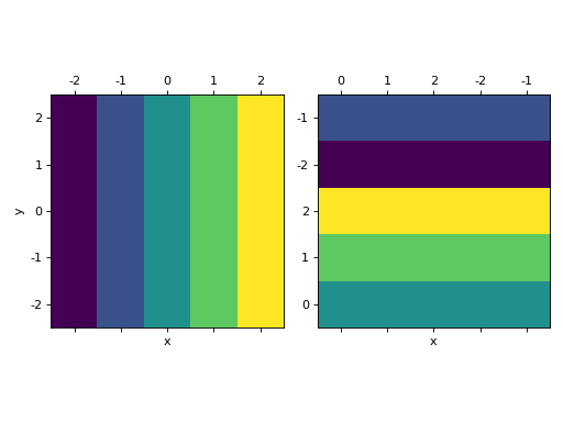
plot_2d_scalar(ax, data, center_origin=True, **kwargs)[source]

Use matshow to plot the (linear) data as a function of space, using the lattice to coordinatize, centering the origin by default.

Parameters

ax (matplotlib axis) – Where to draw the data.
data (torch.tensor) – A single linearized spatial vector.
center_origin (True or False) – If true the origin is centered in the figure.
**kwargs (matshow arguments) – Simply forwarded. origin is fixed to be 'lower'

#!/usr/bin/env python

import matplotlib.pyplot as plt
import tdg

fig, ax = plt.subplots(1,2)

L = tdg.Lattice(5)
L.plot_2d_scalar(ax[0], L.coordinates[:,0])
L.plot_2d_scalar(ax[1], L.coordinates[:,1], center_origin=False)

ax[0].set_xlabel('x')
ax[0].set_ylabel('y')
ax[1].set_xlabel('x')

fig.tight_layout()
plt.show()

(Source code, png, hires.png, pdf)

tdg.LegoSphere

On a square lattice, ‘rotationally symmetric’ has a limited meaning, because the lattice breaks SO(2) in both the UV (via the discretization) and in the IR (via the boundary conditions). However, we still reliably have the smaller \(D_4\) symmetry, and the trivial ireducible representation of \(D_4\) is called \(A_1\). For more details on this symmetry, and exactly why these LegoSpheres are \(A_1\), see D_4 Symmmetry.

class tdg.LegoSphere.LegoSphere(r, c=1)[source]

Bases: H5able

Translationally-invariant potentials in the \(A_1\) representations of the lattice \(D_4\) symmetry can be written as a sum of LegoSpheres,

\[\begin{align} \tilde{V}_{a,a+r} &= \tilde{V}_{0,r} & \tilde{V}_{0,r} &= \mathcal{V} \sum_R \tilde{C}_R \mathcal{S}^R_{0,r} \end{align}\]

where each LegoSphere \(\mathcal{S}\) has a radius \(R\).

To be in the \(A_1\) representation each LegoSphere is a uniformly-weighted stencil with no phases,

\[\begin{align} \mathcal{S}^R_{0,r} &= \frac{1}{\mathcal{N}_R^2} \sum_{g\in D_4} \delta_{r,gR} & \mathcal{S}^R_{ab} &= \frac{1}{\mathcal{N}_R^2} \sum_{g\in D_4} \delta_{b-a,gR} \end{align}\]

where \(g\) acts to rotate spatial displacements on the lattice.

Parameters

r (list or tuple) – the radius given as a vector [x, y]. The magnitude is insufficient information, because two radii with the same magnitude might yield different LegoSpheres (consider [3, 4] and [0, 5], for example).
c (float or a torch.tensor-wrapped number) – the Wilson coefficient \(\tilde{C}_R\).

LegoSpheres may be multiplied by coefficients on either side to give new LegoSpheres with c changed appropriately,

>>> sphere = LegoSphere([0,1], 1.23)
>>> stronger = 2*sphere
>>> stronger.c
tensor(2.4600)

spatial(Lattice)[source]

Parameters: lattice (tdg.Lattice) – a spatial lattice on which to construct \(\tilde{C}_R \mathcal{S}^R_{ab}\)
Returns: a square matrix of dimension [lattice.sites, lattice.sites] where the first index is the superindex \(a\) and the second index is the superindex \(b\).
Return type: torch.tensor

tdg.potential

class tdg.potential.Potential(*spheres)[source]

Bases: H5able

A potential encodes a term in the many-body Hamiltonian like \(nVn\), where \(n\) are number operators and \(V\) can connect different sites.

A potential is built up from one or more LegoSpheres \(\mathcal{S}^{\vec{R}}\), each which carries its own Wilson coefficient \(C_\vec{R}\),

\[\tilde{V} = N_x^2 \sum_R C_R \mathcal{S}^R\]

spatial(lattice)[source]

Parameters: lattice (tdg.Lattice) –
Returns: A matrix encoding \(V\) on the given lattice. The two axes of the matrix are in the order of the lattice coordinates.
Return type: torch.tensor

inverse(lattice)[source]

Parameters: lattice (tdg.Lattice) –
Returns: The inverse matrix of spatial(lattice).
Return type: torch.tensor

eigvals(lattice)[source]

Parameters: lattice (tdg.Lattice) –
Returns: An array of eigenvalues of spatial(lattice). If any of the eigenvalues are imaginary, raises a TypeError; the potential should be Hermitian. Raises a ValueError if any of the eigenvalues are positive; we require the attractive channel.
Return type: torch.tensor

property C0: The Wilson coefficient of the \(\mathcal{S}^0\) piece of the potential.